Limit of a function
| x |  |
|---|---|
| 1 | 0.841471 |
| 0.1 | 0.998334 |
| 0.01 | 0.999983 |
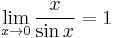
Although the function (sin x)/x is not defined at zero, as x becomes closer and closer to zero, (sin x)/x becomes arbitrarily close to 1. We say that "the limit of (sin x)/x as x approaches zero equals 1."
| Topics in Calculus | ||||||||
|---|---|---|---|---|---|---|---|---|
| Fundamental theorem Limits of functions Continuity Mean value theorem
|
In mathematics, the limit of a function is a fundamental concept in calculus and analysis concerning the behavior of that function near a particular input. Informally, a function f assigns an output f(x) to every input x. The function has a limit L at an input p if f(x) is "close" to L whenever x is "close" to p. In other words, f(x) becomes closer and closer to L as x moves closer and closer to p. More specifically, when f is applied to each input sufficiently close to p, the result is an output value that is arbitrarily close to L. If the inputs "close" to p are taken to values that are very different, the limit is said to not exist. Formal definitions, first devised in the early 19th century, are given below.
Contents
|
History
Although implicit in the development of calculus of the 17th and 18th centuries, the modern notion of the limit of a function goes back to Bolzano who, in 1817, introduced the basics of the epsilon-delta technique to define continuous functions. However, his work was not known during his lifetime (Felscher 2000). Cauchy discussed limits in his Cours d'analyse (1821) and gave essentially the modern definition, but this is not often recognized because he only gave a verbal definition (Grabiner 1983). Weierstrass first introduced the epsilon-delta definition of limit in the form it is usually written today. He also introduced the notations lim and limx→x0 (Burton 1997).
The modern notation of placing the arrow below the limit symbol is due to Hardy in his book A Course of Pure Mathematics in 1908 (Miller 2004).
Motivation
Imagine a person walking over a landscape represented by the graph of y = f(x). His horizontal position is measured by the value of x, much like the position given by a map of the land or by a global positioning system. His altitude is given by the coordinate y. He is walking towards the horizontal position given by x = p. As he does so, he notices that his altitude approaches L. If later asked to guess the altitude over x = p, he would then answer L, even if he had never actually reached that position.
What, then, does it mean to say that his altitude approaches L? It means that his altitude gets nearer and nearer to L except for a possible small error in accuracy. For example, suppose we set a particular accuracy goal for our traveler: he must get within ten meters of L. He reports back that indeed he can get within ten meters of L, since he notes that when he is within fifty horizontal meters of p, his altitude is always ten meters or less from L.
We then change our accuracy goal: can he get within one meter? Yes. If he is within seven horizontal meters of p, then his altitude remains within one meter of the target L. In summary, to say that the traveler's altitude approaches L as his horizontal position approaches p means that for every target accuracy goal, there is some neighborhood of p whose altitude remains within that accuracy goal.
The initial informal statement can now be explicated:
- The limit of a function f(x) as x approaches p is a number L with the following property: given any target distance from L, there is a distance from p within which the values of f(x) remain within the target distance.
This explicit statement is quite close to the formal definition of the limit of a function with values in a topological space.
Definitions
The following definitions (known as (ε, δ)-definitions) are the generally accepted ones for the limit of a function in various contexts.
Functions on the real line
Suppose f : R → R is defined on the real line and p,L ∈ R then we say the limit of f as x approaches p is L and write
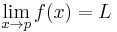
if and only if for every real ε > 0 there exists a real δ > 0 such that 0 < | x - p | < δ implies | f(x) - L | < ε. Note that the value of the limit does not depend on the value of f(p).
A more general definition applies for functions defined on subsets of the real line. Let (a,b) be an open interval in R, and p a point of (a,b). Let f be a real-valued function defined on all of (a, b) except possibly at p. We then say that the limit of f as x approaches p is L if and only if, for every real ε > 0 there exists a real δ > 0 such that 0 < | x - p | < δ and x ∈ (a,b) implies | f(x) - L | < ε. Note that the limit does not depend on f(p) being well-defined.
One-sided limits
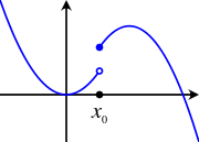
Alternatively x may approach p from above (right) or below (left), in which case the limits may be written as
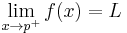
or
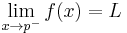
respectively. If both of these limits are equal to L then this can be referred to as the limit of f(x) at p. Conversely, if they are not both equal to L then the limit, as such, does not exist.
A formal definition is as follows. The limit of f(x) as x approaches p from above is L if, for every ε > 0, there exists a δ > 0 such that |f(x) - L| < ε whenever 0 < x - p < δ. The limit of f(x) as x approaches p from below is L if, for every ε > 0, there exists a δ > 0 such that |f(x) - L| < ε whenever 0 < p - x < δ.
If the limit does not exist there is a non-zero oscillation.
Functions on metric spaces
Suppose M and N are subsets of metric spaces A and B, respectively, and f : M → N is defined between M and N, with x ∈ M, p a limit point of M and L ∈ N. We say that the limit of f as x approaches p is L and write
if and only if for every ε > 0 there exists a δ > 0 such that, dB(f(x), L) < ε whenever 0 < dA(x, p) < δ. Again, note that p need not be in the domain of f, nor does L need to be in the range of f.
An alternative definition using the concept of neighbourhood is as follows:
if and only if for every neighbourhood V of L in B there exists a neighbourhood U of p in A, such that f(U∩M - {p}) ⊆ V.
Functions on topological spaces
Suppose X,Y are topological spaces with Y a Hausdorff space. Let p be a limit point of Ω⊆X, and L ∈Y. For a function f : Ω → Y, we say that the limit of f as x approaches p is L (i.e., f(x)→L as x→p) and write
if and only if for every open neighborhood V of L, there exists an open neighborhood U of p such that f(U∩Ω- {p}) ⊆ V. This last part of the definition can also be phrased "there exists an open punctured neighbourhood U of p such that f(U∩Ω) ⊆ V ".
Note that the domain of f does not need to contain p. If it does, then the value of f at p is irrelevant to the definition of the limit. In particular, if the domain of f is X - {p} (or all of X), then the limit of f as x → p exists and is equal to L if and only if for all subsets Ω of X with limit point p the limit of the restriction of f to Ω exists and is equal to L. Sometimes this criterion is used to establish the non-existence of the two-sided limit of a function on R by showing that the one-sided limits either fail to exist or do not agree. Such a view is fundamental in the field of general topology, where limits and continuity at a point are defined in terms of special families of subsets, called filters, or generalized sequences known as nets.
Alternatively, the requirement that Y be a Hausdorff space can be relaxed to the assumption that Y be a general topological space, but then the limit of a function will not be unique. In particular, one can no longer talk about the limit of a function at a point, but rather a limit or the set of limits at a point.
A function is continuous in a limit point p of and in its domain if and only f(p) is the (or, in the general case, a) limit of f(x) as x tends to p.
Limits involving infinity
If the extended real line R is considered, i.e., R ∪ {-∞, ∞}, then it is possible to define limits of a function at infinity.
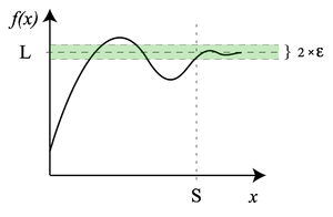
If f(x) is a real function, then the limit of f as x approaches infinity is L, denoted
if and only if for all  there exists S > 0 such that
  whenever x > S.
Similarly, the limit of f as x approaches negative infinity is L, denoted
if and only if for all there exists S < 0 such that whenever x < S.
For example
Limits can also have infinite values, for example the limit of f as x approaches a is infinity, denoted
if and only if for all  there exists
  such that
  whenever
  .
.
These ideas can be combined in an obvious way to produce definitions for different combinations, such as
For example
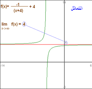
Limits involving infinity are connected with the concept of asymptotes.
These notions of a limit attempt to provide a metric space interpretation to limits at infinity. However, note that these notions of a limit are consistent with the topological space definition of limit if
- a neighborhood of -∞ is defined to contain an interval [-∞, c) where c∈R
- a neighborhood of ∞ is defined to contain an interval (c, ∞] where c∈R
- a neighborhood of a∈R is defined in the normal way metric space R
In this case, R is a topological space and any function of the form f: X → Y with X, Y⊆ R is subject to the topological definition of a limit. Note that with this topological definition, it is easy to define infinite limits at finite points, which have not been defined above in the metric sense.
Alternate notation
Many authors[1] allow for the real projective line to be used as a way to include infinite values as well as extended real line. With this notation, the extended real line is given as R ∪ {-∞, +∞} and the projective real line is R ∪ {∞} where a neighborhood of ∞ is a set of the form {x: |x|>c}. In this notation, for example,
Evaluating limits at infinity for rational functions
There are three basic rules for evaluating limits at infinity for a rational function f(x) = p(x)/q(x):
- If the degree of p is greater than the degree of q, then the limit is positive or negative infinity depending on the signs of the leading coefficients;
- If the degree of p and q are equal, the limit is the leading coefficient of p divided by the leading coefficient of q;
- If the degree of p is less than the degree of q, the limit is 0.
If the limit at infinity exists, it represents a horizontal asymptote at y = L. Polynomials do not have horizontal asymptotes; they may occur with rational functions.
Complex-valued functions
The complex plane with metric  is also a metric space. There are two different types of limits when we consider complex-valued functions.
Limit of a function at a point
If f is a complex-valued function, then
if and only if for all ε > 0 there exists a δ > 0 such that for all real numbers x with  , we have .
It is just a particular case of functions over metric spaces with both M and N are the complex plane.
Limit of a function of more than one variable
By noting that |x-p| represents a distance, the definition of a limit can be extended to functions of more than one variable. In the case of a function f : R2 → R,
- for every ε > 0 there exists a δ > 0 such that for all (x,y) with 0 < ||(x,y)-(p,q)|| < δ, we have |f(x,y)-L| < ε
where ||(x,y)-(p,q)|| represents the Euclidean distance. This can be extended to any number of variables.
Sequential limits
Let f : X → Y be a mapping from a topological space X into a Hausdorff space Y, p∈X and L∈Y.
- The sequential limit of f as x→p is L if and only if, for every sequence (xn) in X which converges to p, the sequence f(xn) converges to L.
If L is the limit (in the sense above) of f as x approaches p, then it is a sequential limit as well, however the converse need not hold in general. If in addition Y is metrizable, then L is the sequential limit of f as x approaches p if and only if it is the limit (in the sense above) of f as x approaches p.
Properties
If the sets A, B, ... form a finite partition of the function domain,  , ... and the relative limit for each of those sets exist and is the equal to, say, L, then the limit exists for the point x and is equal to L. In particular, if f is real-valued, then the limit of f at p is L if and only if both the right-handed limit and left-handed limit of f at p exist and are equal to L.
The function f is continuous at p if and only if the limit of f(x) as x approaches p exists and is equal to f(p). If f : M → N is a function between metric spaces M and N, then it is equivalent that f transforms every sequence in M which converges towards p into a sequence in N which converges towards f(p).
If N is a normed vector space, then the limit operation is linear in the following sense: if the limit of f(x) as x approaches p is L and the limit of g(x) as x approaches p is P, then the limit of f(x) + g(x) as x approaches p is L + P. If a is a scalar from the base field, then the limit of af(x) as x approaches p is aL.
If f is a real-valued (or complex-valued) function, then taking the limit is compatible with the algebraic operations, provided the limits on the right sides of the equations below exist (the last identity only holds if the denominator is non-zero). This fact is often called the algebraic limit theorem.
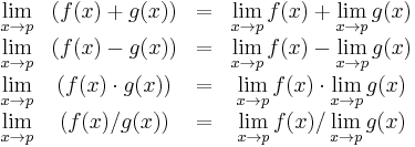
In each case above, when the limits on the right do not exist, or, in the last case, when the limits in both the numerator and the denominator are zero, nonetheless the limit on the left, called an indeterminate form, may still exist—this depends on the functions f and g. These rules are also valid for one-sided limits, for the case p = ±∞, and also for infinite limits using the rules
- q + ∞ = ∞ for q ≠ −∞
- q × ∞ = ∞ if q > 0
- q × ∞ = −∞ if q < 0
- q / ∞ = 0 if q ≠ ± ∞
(see extended real number line).
Note that there is no general rule for the case q / 0; it all depends on the way 0 is approached. Indeterminate forms—for instance, 0/0, 0×∞, ∞−∞, and ∞/∞—are also not covered by these rules, but the corresponding limits can often be determined with L'Hôpital's rule or the Squeeze theorem.
Useful identities
The following rules are valid if the limits on the right hand side exist (and are finite).
 , where S is a scalar multiplier.
 , where b is a positive real number.


 , if the right hand side makes sense; i.e., the two limits on the right exist, and
  .
.
These rules may fail if any of the limits on the right hand side are undefined or infinite.
For example, ![\lim_{n \to \infty} [(3n+2) + (2-3n)] = 4](/I/fa7b6f86a1ceb67a58e2f2f37a3d4403.png) but
but  is undefined.
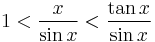
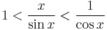
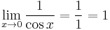
Limits of extra interest
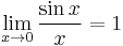
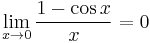
The first limit can be proven with the squeeze theorem. For 0 < x < π/2:

Dividing everything by sin(x) yields
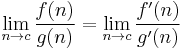
L'Hôpital's rule
This rule uses derivatives and has a conditional usage. (It can only be directly used on limits that "equal" 0/0 or ±∞/±∞. Other indeterminate forms require some algebraic manipulation usually involving setting the limit equal to y, taking the natural logarithm of both sides, and then applying l'Hôpital's rule.)
For example: 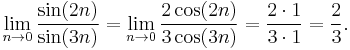
Summations and integrals
A short way to write the limit  is
is  .
.
A short way to write the limit  is
is  .
.
A short way to write the limit  is
is  .
.
See also
- List of limits
- One-sided limit
- Limit of a sequence
- Net (topology)
- Big O notation
- Limit superior and limit inferior
- l'Hôpital's rule
- Squeeze theorem
References
- ↑ For example, "Limit" at Encyclopaedia of Mathematics
- MacTutor History of Weierstrass.
- MacTutor History of Bolzano
- Visual Calculus by Lawrence S. Husch, University of Tennessee (2001)
- Apostol, Tom M., Mathematical Analysis, 2nd ed. Addison-Wesley, 1974. ISBN 0201002884.
- Burton, David M. (1997), The History of Mathematics: An introduction (Third ed.), New York: McGraw-Hill, pp. 558–559, ISBN 0-07-009465-9
- Felscher, Walter (2000), "Bolzano, Cauchy, Epsilon, Delta", American Mathematical Monthly (Mathematical Association of America) 107 (9): 844–862, doi:10.2307/2695743, http://jstor.org/stable/2695743.
- Grabiner, Judith (1983), "Who Gave You the Epsilon? Cauchy and the Origins of Rigorous Calculus", American Mathematical Monthly (Mathematical Association of America) 90 (3): 185–194, doi:10.2307/2975545, http://www.jstor.org/stable/2975545.
- Miller, Jeff (1 December 2004), Earliest Uses of Symbols of Calculus, http://jeff560.tripod.com/calculus.html, retrieved 2008-12-18.
- Page, Warren; Hersh, Reuben; Selden, Annie et al., eds. (2002), Journal "Media Highlights", The College Mathematics (Mathematical Association of America) 33 (2): 147–154, http://www.jstor.org/stable/2687124 Journal.
- Sutherland, W. A., Introduction to Metric and Topological Spaces. Oxford University Press, Oxford, 1975. ISBN 0 19 853161 3.